Randomized Numerical Linear Algebra: Random Projection
Randomized Numerical Linear Algebra: Random Projection
Introduction
Random projection is a method to find the lower rank approximation of matrices in faster time and low error rate. We will see how we can find such a lower rank matrix and its applications in this chapter.
Johnson Lindenstrauss Lemma
Lemma (Johnson Lindenstrauss Lemma [JL84])
Given a set of points \(x_1, x_2, ...., x_n \in \mathcal{R}^d\), there exists a linear mapping \(A\) that creates the images of these points in the target dimension \(k\) such that the pairwise distance between any two points is preserved by the factor \(\epsilon\), where \(k \geq \frac{c\log{n}}{\epsilon^2}, \epsilon > 0\). i.e. for all \((i, j)\)
Note
\(Ax_1, Ax_2, ...., Ax_n \in \mathcal{R}^k\)
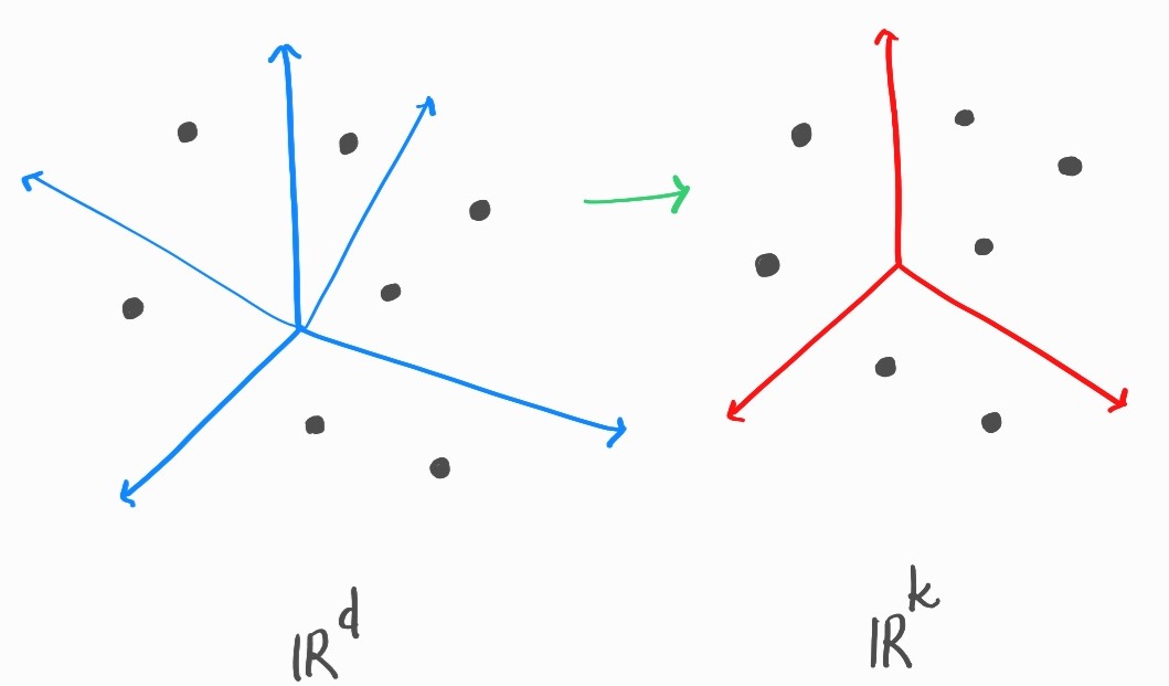
Fig. 43 Projection to Lower Dimension
This mapping is created by filling up the matrix with independant gaussian random variables. The guarantee is that with very high probability for every pair \((i, j)\) the distance \(\|Ax_i - Ax_j\|_2\) will be within \((1 \pm \epsilon)\|x_i - x_j\|_2\).
Other Properties
Remember that a given length \(x\) is preserved with probability \(1 - \delta\) if the target dimension \(k\) is \(\frac{c}{\epsilon^2} \log(\frac{1}{\delta})\)
Property 1
It is known that the bound \(k \geq \frac{c}{\epsilon^2} \log(\frac{1}{\delta})\) is tight.
Property 2
Target dimension depends only on \(\epsilon\) and \(\delta\). It does not depend on the original dimension.
Property 3
Such a result cannot hold on distance metrics other that Euclidean metric. For example, it will not hold for \(L_1\) Norm.
Other Constructions
Earlier Method:
We were creating the matrix \(A\) by creating the matrix \(R\) such that \(R_{ij} \sim N(0, 1)\). We make sure that every column of \(R\) is normalized. So,
We divide by \(\sqrt{k}\) so that the expected norm of each column becomes \(1\).
But it is expensive to sample, create and store Gaussian random variables. We might also need to store floating point numbers. So, instead of using Gaussian random variables the matrix \(R\) is created where:
Definition
where, \(p\) = probability.
Example Application: PCA
Suppose we have \(A \in \mathcal{R}^{n \times d}\). We want a rank-\(k\) approximation \(A'\) such that \(\|A - A'\|_F\) is minimized.
Note
Here, \(\|A - A'\| = \sum_{i, j}(A - A')_{ij}^2\) is the frobenius norm.
The optimal low rank approximation is \(A_k = U_k \Sigma_k V_k^t\), but it takes \(\mathcal{O}(nd \times min(n,d))\) time.
Note
If \(n \approx d\), then it takes \(\mathcal{O}(n^3)\) time.
Low Rank Approximation
We know that \(A_k = P_A^kA\), where projection \(P_A^k = U_kU_k^t\).
Also,
For any \(B\) and \(P_B^k\),
Now, we want \(B\) such that,
It is efficiently computable and small
It leads to low error, i.e. \(\|AA^t - BB^t\| \leq \epsilon\|AA^t\|_2\)
Cheap and Effective Low Rank
For \(A \in \mathcal{R}^{n \times d}\), create \(R \in \mathcal{R}^{d \times k}\) as JL matrix.
Take \(B = AR \in \mathcal{R}^{n \times k}\)
Note
This takes \(\mathcal{O}(ndk)\) time.
Also, \(E[BB^t] = A E[RR^t] A^t = AA^t\), since every \(R_{ij}\) has unit variance and are independent of each other.
JL in Low Rank Approximation
Observe that,
Note
Remember that,
Now, from the JL property,
Using the union bound over a \(\epsilon\) - net, \(k = \tilde{O}(\frac{rank(A)}{\epsilon^2})\)
Note
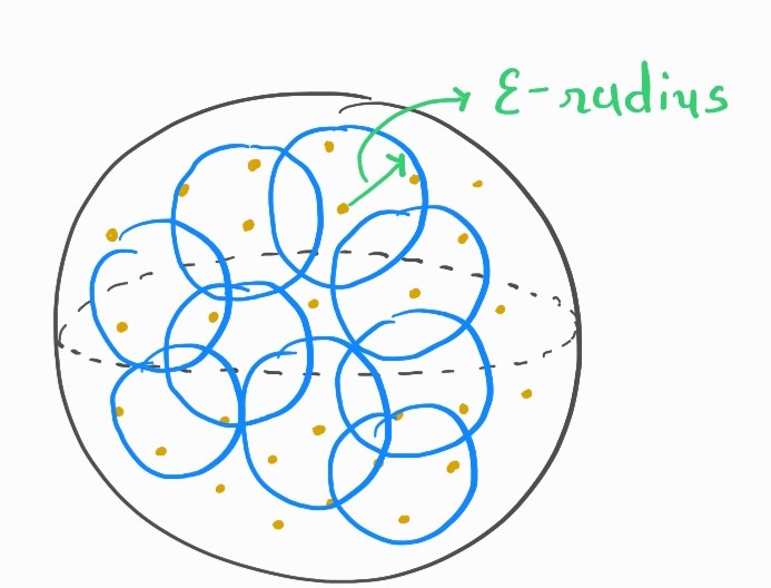
Fig. 44 \(\epsilon\)-net Sphere
\(\epsilon\) - net is when we choose points in unit sphere such that the union of the \(\epsilon\) - radius spheres of all the points give the unit sphere.
We get,
Time taken for Projection
The matrix vector multiplication takes \(\mathcal{O}(kd)\) time, where \(k = \Omega(\frac{1}{\epsilon^2})\).
Now, there is also a lower bound on the target dimension, so can we make the projection faster?
Thought Experiment
Definition
Suppose the projection matrix \(A\) is very sparse:
Now, set \(p\) ~ \(\frac{1}{d}\), then there will be a constant number of entries in most of the rows. So, time taken will be \(\mathcal{O}(dkp)\) ~ \(\mathcal{O}(k)\) only.
Caution
It fails to preserve norm for sparse vectors.
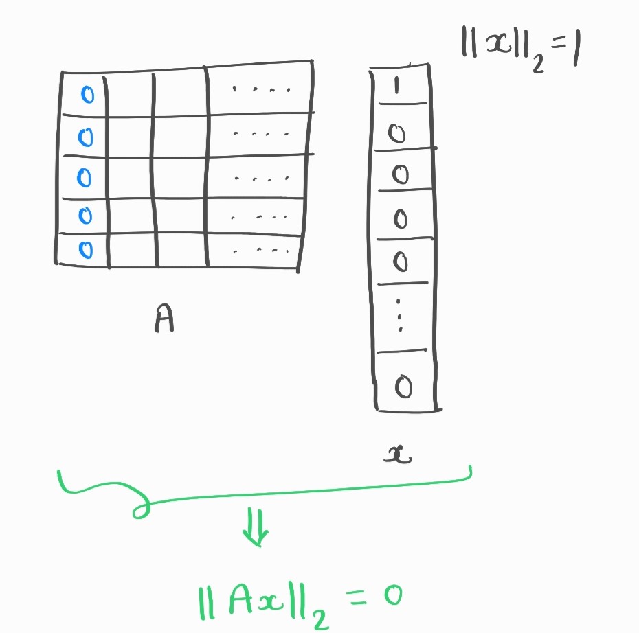
Fig. 45 Example for which norm is not preserved
It works fine if vector is all dense!
We want to be able to work with all vectors. So, we try to preprocess vectors to make them dense.
Note
The time taken for pre-processing should not be more than for projection.
Hadamard Matrices
Definition
Hadamard matrices are defined only when \(d = 2^k\). i.e.
\(H_1 = \begin{pmatrix} 1 \end{pmatrix}\), \(H_2 = \begin{pmatrix} 1 & 1 \\ 1 & -1 \end{pmatrix}\), \(H_{2^{k+1}} = \begin{pmatrix} H_{2^k} & H_{2^k} \\ H_{2^k} & -H_{2^k} \end{pmatrix}\)
Note
Multiplying a vector by \(Hd\) takes \(\mathcal{O}(d\log{d})\) time.
It can be proved by recursion: \(T(d) = 2T(\frac{d}{2}) + \mathcal{O}(d)\)
Densifying using Hadamard
Now, we can use the Hadamard matrix to densify \(x \in \mathcal{R}^d\) as follows:
\(y = HDx\), where \(D \in \mathcal{R}^{d \times d}\) diagonal with,
Here, calculating \(y\) takes \(\mathcal{O}(d\log{d})\) time.
Intuition
\(H\) itself is a rotation,
Sparse vectors are rotated to dense vectors (Uncertainty principle).
But, it is a rotation, it can happen that few dense vectors can become sparse.
Randomization using the diagonal ensures that adversary cannot choose such vectors as input.
Densification Claim
For \(x \in \mathcal{R}^d,\|x\|_2 = 1\),
The maximum is near the average (\(\frac{1}{\sqrt{d}}\)), so the vector \(HDx\) is dense.
Remark
The claim can be proved by applying Cherfnoff style tail inequality per coordinate and union bound.
Projecting a Dense Vector
Take, \(y = HDx\)
\(\max_i \|y_i\| \approx \mathcal{O}(\sqrt{\frac{\log{nd}}{d}})\)
where, \(P \in \mathcal{R}^{k \times d}\) and \(k = \mathcal{O}(\frac{1}{\epsilon^2} \log{\frac{1}{\delta}})\)
And, \(z = PHDx\) is the final projected vector.
Fast JL Transform
If \(q = \mathcal{O}(\|x\|_\infty^2) = \mathcal{O}(\frac{\log{(nd)}}{d})\), \(PHD\) satisfies \(JL\) property.
Observation
Calculating \(y = PHDx\) takes time \(\mathcal{O}(d\log{d} + k\log{(nd)})\), potentially much faster than original Gaussian construction.