Singular Valued Decomposition (SVD)
Singular Valued Decomposition (SVD)
Introduction
The Singular Value Decomposition (SVD) is a basic tool frequently used in Numerical Linear Algebra and in many applications, which generalizes the Spectral Theorem from symmetric n × n matrices to general m × n matrices. We introduce the reader to some of its beautiful properties, mainly related to the Eckart-Young Theorem, which has a geometric nature. The implementation of a SVD algorithm in the computer algebra software Macaulay2 allows a friendly use in many algebro-geometric computations.
Let A be an n × d matrix in d-dimensional space. Consider where subspace is 1-d dimensional For k = 1, 2, 3,…, for the collection of n data points, the singular value decomposition yields the best-fitting k-dimensional subspace.
Let’s start with a one-dimensional subspace, such as a line through the origin. Next the best-fitting k-dimensional subspace may be discovered by k applications of the best fitting line approach, where the best fit line perpendicular to the preceding i-1 lines is found on the i th iteration.When k approaches the rank of the matrix, we have a precise breakdown of the matrix termed the singular value decomposition from these processes.
SVD of a matrix A with real elements is the factorization of A into the product of three matrices, A = UDV T, where the columns of U and V are orthonormal and the matrix D is diagonal with positive real values. The unit length vectors are represented by V’s columns. The coordinates of a row of U will be fractions of the corresponding row of A along each of the lines.
Explanation
Assume that we have a matrix A (nxm) with rank r. Dimensions of rowspace and column space can be atmost n, m respectively. However as the rank of A is r there are excatly r linearly independent row vectors and column vectors, thus the dimension of rowspace and colspace is r.
This means that there are r basis vectors for the rowspace and columnspace.
Note
these basis vectors of rowspace, column space can be found out from the corresponding echelon matrix using non-zero rows and pivot columns.
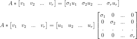
Matrix can be viewed as an operator of linear transformation, each column of a matrix represents a trasformed basis vector. let v be a vector in rowspace of A, then A*v gives a vector in the column space of A. i.e. A v=σ u, σ is a constant.
For the rowspace,there exists some orthogonal basis (say v). we are intrested in finding such basis that gets transformed by A to an orhtogonal basis in colspace.
Note
For a subspace formed by span of vectors, there can be multiple sets of basis vectors. Using algorithm given by Gram-schmidt, an orthogonal basis vectors for the same space can be found using some set of basis vectors.
let v1, v2, v3… vr be that orthogonal basis vectors of the rowspace. u1, u2, u3,…,ur be the transformed vectors that form an orhtogonal basis of the column space,
i.e.
Note
generally in this Σ matrix, σ values are kept in decreasing order, as a consequence the order of v vectors in V and u vectors in V is also changed to maintain the correspondence.
A V=U 𝚺
multiply by V -1 on both sides
A V V -1 =U 𝚺 V -1
A = U 𝚺 V -1
U and V are the collection of orthogonal basis vectors, so U and V are othrogonal matrices. So V VT = I, i.e. V-1 = VT
A = U 𝚺 V T
if we generalize this equation considering all vectors of row and column space, we get
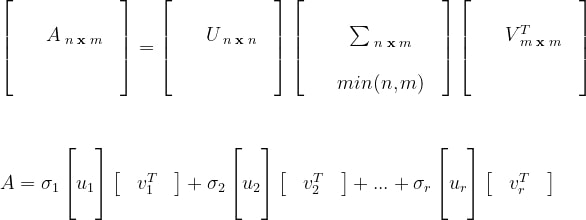
Here ui’s are called left singluar vectors and vi’s are called right singular vectors and σi’s are called singular
Note
when the rank of A is r ( r <= min(n,m)) then we need only first r vectors of U, V. we are able to take only these vectors by manipulating zeroes in matrix 𝚺.
Now let us consider A A T
A A T = (U 𝚺 V T) (U 𝚺 V T)T
= U 𝚺 V T V 𝚺T UT
as 𝚺 is a diagnol matrix 𝚺T=𝚺
= U 𝚺 2 UT
Thus ui’s are eigen vectors of A AT and σi’s are the square roots of eigen values of A AT
Now let us consider A T A
A T A = (U 𝚺 V T)T (U 𝚺 V T)
= V 𝚺T U T U 𝚺 V T
= V 𝚺T U T U 𝚺 V T
= V 𝚺2 VT
Thus vi’s are eigen vectors of AT A and σi’s are the square roots of eigen values of AT A
***Property: Matrices (AB) and (BA) have same eigen values.
Top K Truncated SVD:
use first k vectors of U, V and the corresponding spectral values (top k x k submatrix of Σ )
Implementation of SVD
import numpy as np

A = np.array([[7, 2], [3, 4], [5, 3]])
U, D, V = np.linalg.svd(A)  # actually V here = V (Transpose) in svd
U, D, V
(array([[-0.69366543,  0.59343205, -0.40824829],
        [-0.4427092 , -0.79833696, -0.40824829],
        [-0.56818732, -0.10245245,  0.81649658]]),
 array([10.25142677,  2.62835484]),
 array([[-0.88033817, -0.47434662],
        [ 0.47434662, -0.88033817]]))
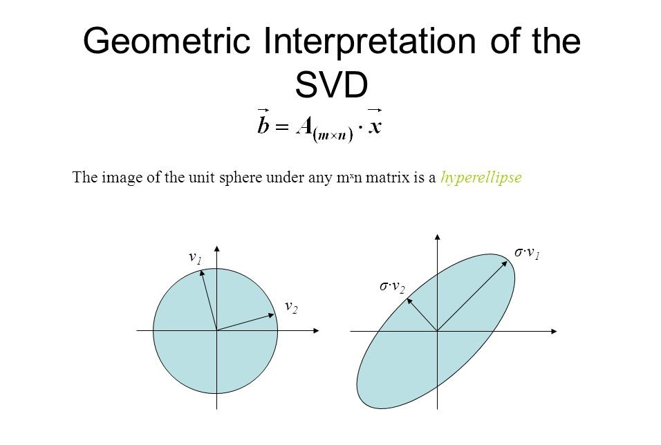
Fig credit: Math for CSLecture
The above image shows how the points get linearly transformed by A, i.e. A v= σ u (equation 1)
svd says 3 important things about this transormation
The ui vectors in SVD decompostion of A form the axes of the new transformed subspace
the length of each axis is equal to coressponding σi value
the preimage of ui is the corresponding vi of the SVD of A (from equation 1)
References:
“Spectral Learning on Matrices and Tensors” textbook