Applications of SVD
Applications of SVD
Implementation of SVD
import numpy as np

A = np.array([[7, 2], [3, 4], [5, 3]])
U, D, V = np.linalg.svd(A)  # v here=v(Trans) in svd transpose actually
U, D, V
(array([[-0.69366543,  0.59343205, -0.40824829],
        [-0.4427092 , -0.79833696, -0.40824829],
        [-0.56818732, -0.10245245,  0.81649658]]),
 array([10.25142677,  2.62835484]),
 array([[-0.88033817, -0.47434662],
        [ 0.47434662, -0.88033817]]))
Applications of Singular Value Decomposition (SVD)
Image Compression
import numpy as np
import matplotlib.pyplot as plt

# This line is required to display visualizations in the browser
%matplotlib inline
from skimage import data
from skimage.color import rgb2gray
from ipywidgets import interact, interactive, interact_manual
from skimage import img_as_ubyte, img_as_float

gray_images = {
    "cat": rgb2gray(img_as_float(data.chelsea())),
    "astro": rgb2gray(img_as_float(data.astronaut())),
    "camera": data.camera(),
    "coin": data.coins(),
    "clock": data.clock(),
    "blobs": data.binary_blobs(),
    "coffee": rgb2gray(img_as_float(data.coffee())),
}
from numpy.linalg import svd
def compress_svd(image, k):
    """
    Perform svd decomposition and truncated (using k singular values/vectors) reconstruction
    returns
    --------
      reconstructed matrix reconst_matrix, array of singular values s
    """
    U, s, V = svd(image, full_matrices=False)
    reconst_matrix = np.dot(U[:, :k], np.dot(np.diag(s[:k]), V[:k, :]))

    return reconst_matrix, s
def compress_show_gray_images(img_name, k):
    """
    compresses gray scale images and display the reconstructed image.
    Also displays a plot of singular values
    """
    image = gray_images[img_name]
    original_shape = image.shape
    reconst_img, s = compress_svd(image, k)
    fig, axes = plt.subplots(1, 2, figsize=(8, 5))
    axes[0].plot(s)
    compression_ratio = (
        100.0
        * (k * (original_shape[0] + original_shape[1]) + k)
        / (original_shape[0] * original_shape[1])
    )
    axes[1].set_title("compression ratio={:.2f}".format(compression_ratio) + "%")
    axes[1].imshow(reconst_img, cmap="gray")
    axes[1].axis("off")
    fig.tight_layout()
import numpy as np


def compute_k_max(img_name):
    """
    utility function for calculating max value of the slider range
    """
    img = gray_images[img_name]
    m, n = img.shape
    return m * n / (m + n + 1)


# set up the widgets
import ipywidgets as widgets

list_widget = widgets.Dropdown(options=list(gray_images.keys()))
int_slider_widget = widgets.IntSlider(min=1, max=compute_k_max("cat"))


def update_k_max(*args):
    img_name = list_widget.value
    int_slider_widget.max = compute_k_max(img_name)


list_widget.observe(update_k_max, "value")
interact(compress_show_gray_images, img_name=list_widget, k=int_slider_widget);
Reference :https://colab.research.google.com/drive/1HLJcLzWG46NlPMCgD_KdVLCl-k68mVp2#scrollTo=d35EdHEQpv-b
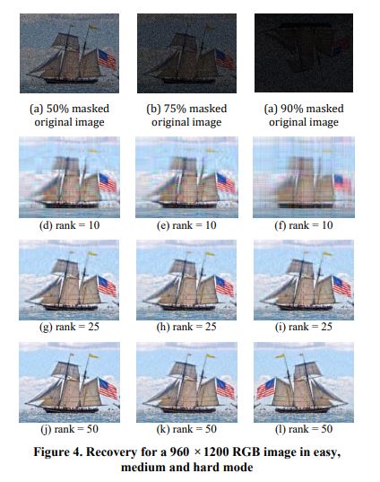
Image Recovery
The process of filling in the missing items in a partly seen matrix is known as matrix completion. A well-known example of this is the Netflix dilemma.If customer I has viewed movie j and is otherwise unavailable, we’d want to anticipate the remaining entries in order to offer appropriate suggestions to consumers on what to watch next, given a ratings matrix in which each entry (i,j) indicates the rating of movie j by customer i.
The fact that most users have a pattern in the movies they view and the ratings they give to these movies is a key factor in resolving this issue. As a result, the ratings matrix contains very little unique data. This implies that a low-rank matrix would be able to approximate the matrix well enough.
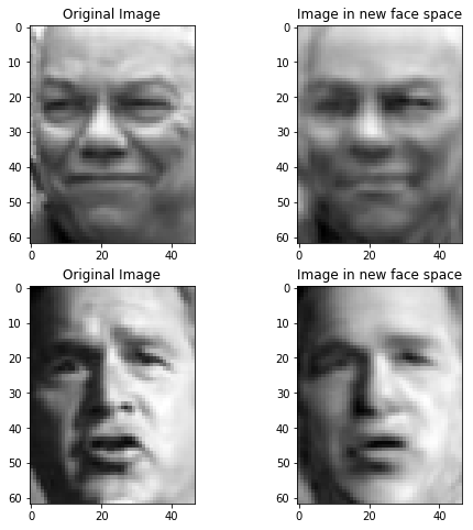
Eigen faces
The encoding is accomplished by expressing each face in the new face space as a linear combination of the specified eigenfaces.
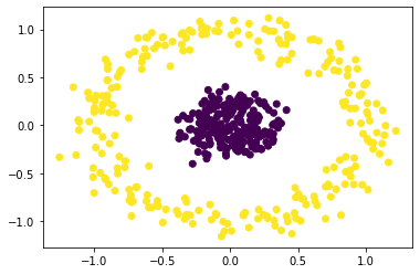
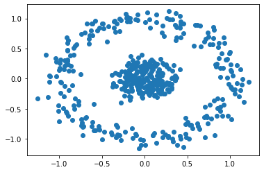
Spectral Clustering
from sklearn.datasets import make_circles
from sklearn.neighbors import kneighbors_graph
from sklearn.cluster import SpectralClustering
import numpy as np
import matplotlib.pyplot as plt

# generate your data
X, labels = make_circles(n_samples=500, noise=0.1, factor=0.2)

# plot your data
plt.scatter(X[:, 0], X[:, 1])
plt.show()

# train and predict
s_cluster = SpectralClustering(
    n_clusters=2, eigen_solver="arpack", affinity="nearest_neighbors"
).fit_predict(X)

# plot clustered data
plt.scatter(X[:, 0], X[:, 1], c=s_cluster)
plt.show()
# source :Gitgub - rawspectral_clustering.py
D:\anaconda\lib\site-packages\sklearn\manifold\_spectral_embedding.py:245: UserWarning: Graph is not fully connected, spectral embedding may not work as expected.
  warnings.warn("Graph is not fully connected, spectral embedding"