Clustering
Contents
Clustering
Clustering is one of the forms of unsupervised learning when the data does not have labels.
It is useful for:
Detecting patterns
Example - In image data, customer shopping results, anomalies, etc.Optimizing
Example - Distributing data across various machines, cleaning up search results, facility allocation for city planning, etc.When we ‘don’t know’ what exactly we are looking for
Basic idea
Clustering is basically concerned with grouping the objects into a small number of meaningful groups called clusters.
However-
How do we define the similarity/distance between the objects?
When do we call the groups meaningful?
How many groups should the objects be divided into?
So typically, there is no supervision for clustering the objects. Since there is no ground truth, evaluating the quality of clustering is often difficult.
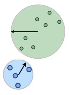
For example, consider the two clustering cases depicted in the figure 1.3 below:
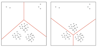
What is the right way of clustering - the left or the right? Essentially, the answer depends on the application in use. However, most times, clustering might not have an end goal and there might not be a fixed application to proceed with. In such a case, to define what the right way of clustering is, we need an objective function!
Caution
There is no unique way of defining clusters that work for all applications.
Objective Function
The most structured way to cluster the objects is the following:
Specifying the number of clusters required
K centers / K means / K-medianSpecifying cluster separation or quality
Dunn’s index - works on the notion of density, i.e., a set of points would be called a cluster if the points are dense enough
Radius - works on the notion of radius of the cluster, i.e., a set of points would count as a cluster if all the points fall within certain radius from a specific centerGraph-based measures
This extends the objects of clusters from being points to networks. For example, what would the shortest distance mean with respect to networks? Is it the shortest path between the nodes?Working without an objective function
Hierarchical clustering schemes that define clusters based on some intuitive algorithms
K-Center
Introduction
Consider a cluster with specific cluster centers.
Cost of a point = Distance of the point from the closest cluster center
Cost of a single cluster = Maximum of all the point costs of that cluster
Cost of a complete clustering = Maximum of all the cluster costs, say D
Example:
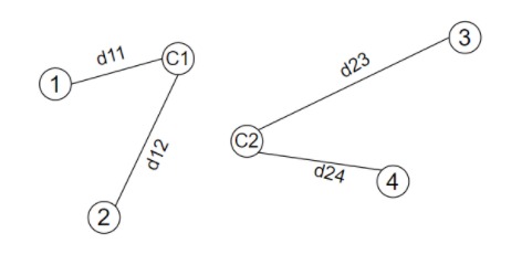
Cost of points:
Point 1 = \(d_{11}\)
Point 2 = \(d_{12}\)
Point 3 = \(d_{23}\)
Point 4 = \(d_{24}\)
Cost of clusters:
Cluster 1 = max(\(d_{11}\) , \(d_{12}\) ) = \(d_{12}\)
Cluster 2 = max(\(d_{23}\) , \(d_{24}\) ) = \(d_{23}\)
Cost of clustering:
D = max(\(d_{12}\) , \(d_{23}\) ) = \(d_{23}\)
Algorithm’s Goal: The algorithm has to find the centers \(C_1\) , \(C_2\) such that the total cost of the clustering(D) is minimized, i.e., the distance of the farthest point from the center is minimized.
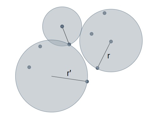
Consider a set of points as shown in the image. The aim is to choose the positions of k number of centers and create circles corresponding to each center such that all the points in the set lie inside the k circles.
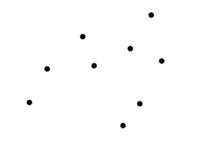
K = 4
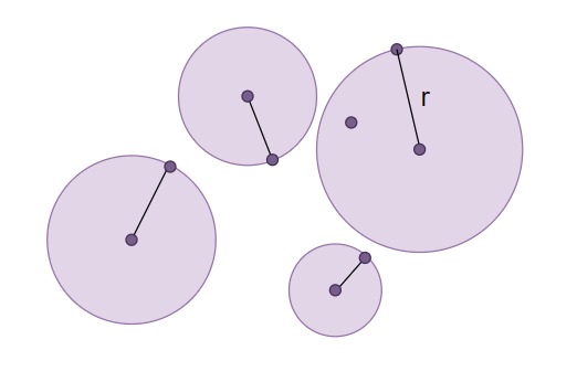
Solution #1:
All four centers are the points of the input set. The radii correspond to the distance of the farthest points from the centers.
Notice that the cost of the cluster(D) = r
Solution #2:
All the centers of the circles need not be the points from the input set, but can be arbitrary. Also, although k=4, only three circles have been used to enclose all the points.
However, notice that the cost of the new cluster(D’) = r’ > r
Observations
The input set of points should be enclosed in utmost k circles
The algorithm gets to choose the centers of the circles
All the points should be covered within the circles
Solution value(cost) is given by the largest radii among all the circles
If we are allowed to k circles, is it possible to obtain a better solution by using k-1 circles instead of k circles? No, because we can always split the biggest ball into two to reduce the cost. It means, given the k centers, we will always use all of them for the optimal solution.
This simple problem of finding optimal K-balls is NP-hard.
However, there is a solvable algorithm. It is an easy 2-approximation, i.e., if the most optimal solution using at most k circles needs a maximum radius OPT, then our algorithm which also uses k circles will have a maximum radius of not more than 2 \(*\) OPT.
Algorithm 1 (2-Approximation Algorithm)
Let the input set \(V\) contain a total of ‘n’ points.
Let all the ‘k’ centers be the points of the input set and are in set \(C\) .
Following is the pseudocode for 2-approximation:
Choose a point \(v\) \(\in \) \(V\) arbitrarily and make it first center \(c_1\) .
For every point \(v \in V\) compute \(d_1[v]\) from \(c_1\) .
Pick the point \(c_2\) with highest distance from \(c_1\) and add it to the \(C\).
Continue till the \(K\) centers are found.
Runtime: \(O(kn) \)
Why 2-approximation?
Suppose \(D\) is th largest radius among K-Centers.
Let,
g(1), g(2), … … g(k) = k centers
g(k+1) = farthest point from {g(1), g(2), …..g(k)}
G(i) = {g(1), g(2), … g(i)}
G(k) = final set
Solution cost = d (g(k+1) , G(k))
\( \Delta (i) \) = max of d(x, G(i)) i.e farthest from G(i)}
Lemma 1
\( \Delta (i+1) \le \Delta (i)\)
Proof. \( \Delta (i+1) =\) max of d (x, G(i)) = d (g(i+1), G(i))
Also, d(g(i+1), G(i)) \(\le\) d(g(i+1), G(i-1)) … Since our algorithm is greedy
Now, d(g(i+1), G(i-1)) \(\le\) d(g(i), G(i-1)) = \(\Delta (i) \)
Hence \( \Delta (i+1) \le \Delta (i)\)
Lemma 2
For any two \(i, j\) where \( j < i\),
Proof. d(g(i), g(j)) \(\ge\) d(g(i), G(i-1)) = \(\Delta (i)\)
Also, \( \Delta (i) \ge \Delta (k) \) … from previous lemma
Putting these together for any i, j
d(g(i), g(j)) \(\ge \Delta _{min} (i, j) \ge \Delta (k)\)
d(g(k+1), g(i)) \( \ge \) d(g(k+1), G(k)) = \( \Delta (k)\)
Hence, when we consider G(k+1), all pairs of points in G(k+1) are separated by atleast \(\Delta (k)\)
Lemma 3
Suppose \(O\) be the K-Centers of the optimal solution and the associated cost be \( \Delta (O)\) , then
Proof. Take the points in the set H(k+1) = { h(1), h(2), …. , h(k+1)}
Since we have k circles and K+1 balls, there must be atleast two of these points in the same circle. (Pigeonhole Principle)
say x and y are mapped to the same center c.
max(d(x, c), d(y, c)) \( \le \Delta (O) \)
Since x, y \(\in \) G(k+1),
Important
Can We Do Better?
We can do no better than the 2-approximation.
For any small constant 𝜖 > 0, we cannot get a 2 - 𝜖 approximation, unless P = NP.
If the distance function does not obey triangle inequality, then we cannot build any algorithm for any arbitrary constant factor approximation, unless P = NP. For specific distance functions and datasets, we might get good heuristics.
K-Means
Objective Function
The distance function is typical \(L_2\).
Let the set of centers to be generated by the algorithm be C = {\(c_1, c_2, c_3, ...., c_k\)}
Let the cost of this set C be given by:
cost(C) = \( \Sigma _x \text{ } min_{cx} d(x, cx)^2\)
For each point x, choose the closest center \(c_x\) i.e., the Euclidean distance d( ) between x and \(c_x\) is the minimum. The cost takes the summation of the squares of all the minimum distances from points to the centers.
Find the set C to optimize the cost
Leads to natural partitioning of the data
There is a huge amount of work, both from theory and data mining community
Great example of divergence between theory and practice and how that prompted new research directions for both
K Means Objective: Alternative View
We define the ‘best’ k-clustering of the data by minimizing the variance of each cluster. The mean and variance of each cluster are given by the following:
Mean: \( c_i = \frac {1}{|c_i|} \Sigma _{x \in c_i} x\)
It refers to the expected location of a point in the cluster
Variance = \( \Sigma _{x \in c_i} ||x-c_i||^2\)
Connection with Maximum Likelihood Function
Let us now study the maximum likelihood motivation and see how it is related to the k-means criterion. Consider the input data set of points {\( x_1, x_2, …, x_k \)} and a Gaussian Probability Density Function(PDF) with its parameters μ and \( \sigma ^2 \).
For the given Gaussian parameters, the likelihood function would imply the probability of the points \( x_1, x_2, …, x_k \) to fit the Gaussian family with the center μ and covariance matrix \(\sigma ^2I\) . This probability is given by:
On taking the logarithm of this probability likelihood function, we obtain:
The first term on the right hand side denotes nothing but the cost of the cluster.
Therefore, the log likelihood of fitting the points of the input set to a Gaussian distribution with parameters μ and \(\sigma ^2\) is proportional to the k-means cost of the cluster of these points assigned to the center at μ summed with some constant function of \(\sigma \).
Voronoi Partition
When we talk about clustering, there are two ways of looking at it:
We create partitions among the data points to divide the set into smaller clusters
We pick few points as representative centers and add the nearest points to these representatives to their cluster
However, it turns out that both of these ways have one-to-one correspondence and that they are both basically similar.
To understand this better, consider a set of points of which \(c_1, c_2, \text{and }c_3 \) are chosen as the centers. The two ways of viewing clustering mentioned above are now related this way - if we create a partitioning as shown in the figure, it would mean that all the points in the partitioned regions I, II, and III are closer to nothing but the centers \(c_1, c_2, \text{and }c_3 \) respectively.
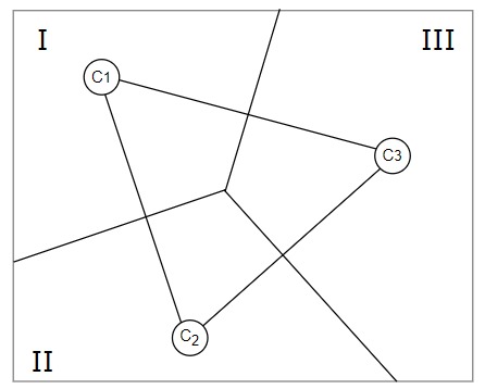
Notice how the partitioning is achieved. Each line(or hyperplane) partitioning two centers is the perpendicular bisector of the line joining the respective centers. This method of partitioning is called Voronoi Partition.
As a next step, it is important to understand the number of partitions that are to be created in order to achieve the desired cluster. The reason being that the performance of the algorithm for K-means clustering in the worst case would be bounded by the number of partitions.
It turns out that to Voronoi partition an input data set of n points with k chosen centers, we need \(n^{k-1}\) partitions. Although this number of partitions appears fair for smaller sets, the number would crash as n and k begin to increase.
Center vs Partitioning
We have seen that given a set of points and some specified centers, we have partitioned the data using Voronoi Partitioning. Now consider a case that goes the other way - suppose we are given a set of points already partitioned with the centers unspecified. In this case, which point would be the optimal center in each partition?
Coming up with a center of a partition \(C_i\) would mean that we need to find a point μ in \(C_i\) such that the value \(\sum _{x\in c_i}|x-\mu|^2\) is minimized. Therefore, the center(μ) has to be the mean of all the points in the partition.
Now that we know how to partition the set of points given the centers and also to find the centers given the partitions of the input set, we next understand Lloyd’s algorithm.
Algorithm 2 (Lloyd’s Algorithm )
Llyod’s is an iterative algorithm that keeps iterating on the following steps:
Find the current centers of the partitions
Assign the points to the nearest centers
Recalculate centers and partition the set of points through Voronoi
But when should this iterative loop terminate? Following are the stopping criteria for the Llyod’s iteration:
The cluster centers do not shift much
When none or only few points change the cluster(move from one partition to the next)
Lloyd’s Algorithm: Analysis
Given a set of N points with k centers in a d-dimensional space:
The time taken to calculate new cluster assignments is of the order O(kNd)
That is, for each of the N points, the distance has to be calculated from each of the k centers using all d coordinates to find the closest center.The time taken to calculate the new centers follows the order of O(Nd)
Consider a cluster of three partitions with \(n_1\), \(n_2\), and \(n_3\) points in each partition. To find the center of each partition(equivalent to calculating the mean of all the points of a partition), \(n_1d\), \(n_2d\), and \(n_3d\) time would be required. Therefore the total time (\(n_1+n_2+n_3\))d would scale to Nd.