Flajolet-Martin Sketch

Flajolet-Martin Sketch¶

Introduction¶

Flajolet-Martin Sketch, popularly known as the FM Algorithm, is an algorithm for the distinct count problem in a stream. The algorithm can approximate the distinct elements in a stream with a single pass and space-consumption logarithmic in the maximal number of possible distinct elements in the stream

The Algorithm¶

We are given a random hash function that maps the elements of the universe to integers in the range 0 to $2^l-1$.

\[h(x) : U → [0,2^l-1]\]

The output of this hash function can be stored using a $l$-length bit string.

Note

We assume the outputs to be sufficiently uniformly distributed and that the hash function is completely random.

Definition

We define the zeros of a number as the index of the first non-zero bit from the right in the binary representation of that number with 0-indexing. It is simply the number of zeros at the end of the bit string. It can be defined as the maximum power of 2 that divides the number.

\[ zeros(v) = max\{i, 2^i \text{ divides } v\} \]

Example:
$zeros(1011000) = 3$, here the maximum power of 2 which will divide the number is 3
$zeros(0010010) = 3$, here the maximum power of 2 which will divide the number is 1

Note

$zeros(0000000)$ will be equal to 0 and not 7.

Next, we need to find out the maximum number of zeros an element has in the input stream. We can calculate the maximum zeros as follows in the same pass of the stream:

Initialize z as 0.
For each element $x$ in stream:

if $zeros(h(x)) > z$, $z ← zeros(h(x))$

Finally, we return the estimate of the number of distinct elements in our stream as:

\[ \text{Number of distinct elements} = 2^{z+\frac{1}{2}} \]

Note

The addition of half in the final estimate of distinct count is due to the correction factor is found out by calculations. It can be seen in the original article by Flajolet and Martin.

Example of the Algorithm:¶

Suppose we need to calculate the number of distinct elements in the following stream:

Fig. 40 After the hash function, suppose the elements are mapped as followed:¶

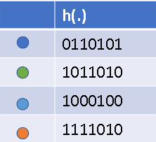
Fig. 41 The maximum number of zeros in the outputs of the hash map is equal to 2. Thus our estimate will be equal to: $ \text{Distinct count} = 2^{2+0.5} ≈ 6 $¶

Thus, the algorithm returns 6 as the number of distinct elements in our stream. The answer is not accurate and this is because we have a very small stream. The algorithm gives better results for bigger datasets.

Note

The above algorithm was further refined in LogLog and HyperLogLog algorithms to improve accuracy.

Proof of correctness for Flajolet-Martin Sketch¶

Basic intuition¶

The main intuition behind the algorithm is that suppose we choose $n = 2^k$ elements uniformly random from $[0,N]$ then we expect the number of elements to be divisible

by $2$ to be $\frac{n}{2}$, i.e., $2^{k-1}$
by $4$ to be $\frac{n}{4}$, i.e., $2^{k-2}$
$…$
Similary, by $2^{k-1}$ to be $2$
by $2^k$ to be $1$
by $2^{k+1}$ to be $\frac{1}{2}$

Therefore we don’t expect any number to be divisible by $2^{k+1}$

Now, for a number to be divisible

by 2 it must have atleast 1 trailing zero in its binary representation
…
by 4 it must have atleast 2 trailing zeros in its binary representation
Similarly, by $2^{k}$ it must have atleast $k$ trailing zeros in its binary representation

Since we don’t expect any number to be divisible by $2^{k+1}$, we do not expect $k+1$ trailing zeros. We expect the maximum number of trailing zeros in the input to be $k$ since we have $n=2^k$.

Therefore in the algorithm we find the maximum number of trailing zeros and return $2^{z+\frac{1}{2}}$.

Note

Probability that an element is divisible

by $2 \text{ is } \frac{\text{number of elements divisible by 2}}{total elements} = \frac{2^{k-1}}{2^k} = 2^{-1}$
Similarly, by $4 \text{ is } 2^{-2}$
…
by $2^r \text{ is } 2^{-r}$

Formalizing our Intuition¶

Let $S$ be the set of elements that appeared in the stream.

Let $zeros(x)$ be the number of trailing zeros $x$ has.

For any $r \in [l], j \in U$ let $X_{rj} = \text{indicator of }zeros(h(j)) \ge r$

\[\begin{split} \begin{equation} \tag{1} X_{rj} = \begin{cases} 1 & \text{when $zeros(h(j)) \ge r$} \\ 0 & \text{else} \end{cases} \end{equation} \end{split}\]

Now, $P[zeros(h(j)) \ge r]$ is same as $P[ \text{element is divisible by }2^r]$, that is, $2^{-r}$

\[\begin{split} \therefore \begin{equation} \tag{2} X_{rj} = \begin{cases} 1 & \text{w.p. $2^{-r}$} \\ 0 & \text{else} \end{cases} \end{equation} \end{split}\]

Let $Y_r = \text{number of }j \in U \text{such that }zeros(h(j)) \ge r$

\[ \therefore Y_r = \sum_{j \in S}{X_{rj}} \]

Let $\hat{z}$ be the final value of $z$ after algorithm has seen all the data. That is the maximum value of trailing zeros.

Now, if we have $Y_r>0$ then, we have atleast one element $j$ such that $zeros(h(j)) \ge r$. Therefore, $\hat{z} \ge r$ if $Y_r>0$.

Equivalentely, if we have $Y_r=0$, then we do not have any element that has more than $r$ trailing zeros. Therefore $\hat{z} < r$ if $Y_r=0$.

Now, we find $E[Y_r]$.

\[ \begin{align}\begin{aligned}\begin{split} \therefore E[Y_r] = E[\sum_{j \in S}{X_{rj}}] \\\end{split}\\\begin{split}\therefore E[Y_r] = \sum_{j \in S}{E[X_{rj}]} \\ \end{split}\\\begin{split}\text{Now, } E[X_{rj}] = 1 \times 2^{-r} = 2^{-r} \\\end{split}\\\therefore E[Y_r] = \sum_{j \in S}{2^{-r}} = \frac{n}{2^r} \end{aligned}\end{align} \]

Now, we find $var(Y_r)$.

\[ \begin{align}\begin{aligned}\begin{split} \therefore var(Y_r) = \sum_{j \in S}{var(X_{rj})} \\\end{split}\\\begin{split}\therefore var(Y_r) = \sum_{j \in S}{E[(X_{rj} - E[X_{rj}])^2])} \\\end{split}\\\begin{split}\therefore var(Y_r) \le \sum_{j \in S}{E[X_{rj}^2]} \\\end{split}\\\begin{split}\text{($X_{rj}^2$ and $X_{rj}$ have the same probablity distribution.)} \\\end{split}\\\begin{split}\therefore var(Y_r) \le \sum_{j \in S}{2^{-r}} \\\end{split}\\\begin{split}\therefore var(Y_r) \le \frac{n}{2^r} \\ \end{split}\end{aligned}\end{align} \]

Therefore, we have $E[Y_r] = \frac{n}{2^r}$ and $var(Y_r) \le \frac{n}{2^r}$

Now, we find $P[Y_r > 0]$ and $P[Y_r = 0]$.

Since $Y_r$ is a count of elements, $Y_r > 0$ means $Y_r \ge 1$.

By Markov inequality,

\[ \begin{align}\begin{aligned}\begin{split} P[Y_r\ge1] \le \frac{E[Y_r]}{1} \\\end{split}\\\begin{split}\therefore P[Y_r \ge 1] \le \frac{n}{2^r} \\\end{split}\\\therefore P[Y_r > 0] = \frac{n}{2^r} \end{aligned}\end{align} \]

Now, $Y_r = 0$ means that it is its expectation away from its expectation. That is, $|Y_r - E[Y_r]| \ge E[Y_r]$

\[ \therefore P[Y_r = 0] = P[|Y_r - E[Y_r]| \ge E[Y_r]] \]

Using Chernoff bound,

\[ \begin{align}\begin{aligned}\begin{split} P[|Y_r - E[Y_r]| \ge E[Y_r]] \le \frac{var(Y_r)}{E[Y_r]^2} \\\end{split}\\\begin{split}\text{Since } var(Y_r) \le \frac{n}{2^r} \\\end{split}\\\begin{split}\therefore P[|Y_r - E[Y_r]| \ge E[Y_r]] \le \frac{2^r}{n} \\\end{split}\\\therefore P[Y_r = 0] \le \frac{2^r}{n} \end{aligned}\end{align} \]

Upper bound¶

Let the returned estimate of FM algo be $\hat{n}=2^{\hat{z}+0.5}$.

Let $a$ be the smallest integer such that $2^{a+0.5} \ge 4n$, where $n$ is the actual number of distinct elements.

We want to find the probability that our estimate is greater that 4 times the actual value, i.e., $P[\hat{n} \ge 4n]$

\[ \begin{align}\begin{aligned}\begin{split} \therefore \hat{n} \ge 4n \implies \hat{z} \ge a \\\end{split}\\\begin{split}\therefore P[\hat{n} \ge 4n] = P[\hat{z} \ge a] \\ \end{split}\end{aligned}\end{align} \]

$\hat{z} \ge a$ means that there are one or more elements, $j$, with $zeros(h(j)) \ge a$. Therefore, $Y_a > 0$. Thus, $P[\hat{z} \ge a] = P[Y_a > 0]$

\[ \begin{align}\begin{aligned}\begin{split} \therefore P[Y_a > 0] \le \frac{n}{2^a} \\\end{split}\\\begin{split}\therefore P[Y_a > 0] \le \frac{\sqrt{2}}{4} \le 0.35 \\\end{split}\\\therefore P[\hat{n} \ge 4n] \le 0.35 \end{aligned}\end{align} \]

Lower bound¶

Let the returned estimate of FM algo be $\hat{n}=2^{\hat{z}+0.5}$.

Let $b$ be the largest integer such that $2^{b+0.5} \le \frac{n}{4}$, where $n$ is the actual number of distinct elements.

We want to find the probability that our estimate is greater that 4 times the actual value, i.e., $P[\hat{n} \le \frac{n}{4}]$

\[ \begin{align}\begin{aligned}\begin{split} \therefore \hat{n} \le \frac{n}{4} \implies \hat{z} \le b \\\end{split}\\\begin{split}\therefore P[\hat{n} \le \frac{n}{4}] = P[\hat{z} \le b] \\ \end{split}\end{aligned}\end{align} \]

$\hat{z} \le b$ means that there are no elements, $j$, with $zeros(h(j)) = b+1$. Therefore, $Y_{b+1} = 0$. Thus, $P[\hat{z} \le b] = P[Y_{b+1} = 0]$

\[ \begin{align}\begin{aligned}\begin{split} \therefore P[Y_{b+1} = 0] \le \frac{2^{b+1}}{n} \\\end{split}\\\begin{split}\therefore P[Y_{b+1} = 0] \le \frac{\sqrt{2}}{4} \le 0.35 \\\end{split}\\\therefore P[\hat{n} \le \frac{n}{4}] \le 0.35 \end{aligned}\end{align} \]

Understanding the bounds¶

From union bound, we get that

\[ \begin{align}\begin{aligned}\begin{split} P[\frac{n}{4} \le \hat{n} \le 4n] \ge 1 - 0.35 - 0.35 \\\end{split}\\\therefore P[\frac{n}{4} \le \hat{n} \le 4n] \ge 0.3 \end{aligned}\end{align} \]

Improving the probabilities¶

The probability we obtain is not very good since we only say with $30\%$ certainity that our estimate lies between $\frac{n}{4}$ and $4n$.

Therefore we apply the Median of Estimates trick to improve our probabilities.

Median of Estimates¶

We create $\hat{z_1}, \hat{z_2}, \dots \hat{z_k}$ estimates in parallel and then return the median of them.

From the $k$ estimates, we expect $35\%$ of them to exceed $4n$. But for the median to exceed $4n$ we need atleast $\frac{k}{2}$ to exceed $4n$. From the Chernoff inequality, we can show that

\[ \begin{align}\begin{aligned}\begin{split} P[median > 4n] = exp(-\Omega(k)) \\\end{split}\\Similarly, P[median < \frac{n}{4}] = exp(-\Omega(k)) \end{aligned}\end{align} \]

Therefore, $P[\frac{n}{4} \le median \le 4n] = 1-exp(-\Omega(k))$

Therefore, given an error probability $\delta$ we choose $k=O(log(\frac{1}{\delta}))$

Median of Means¶

To make our estimate within $1 \pm \epsilon$, with probability $1-\delta$,

We first make $\frac{1}{\epsilon^2}log(\frac{1}{\delta})$ copies of our algorithm. And find $\frac{1}{\epsilon^2}log(\frac{1}{\delta})$ estimates.
Then find mean of $\frac{1}{\epsilon^2}$ estimates.
then we take median of $log(\frac{1}{\delta})$ such estimates.

Linear Counting

Finding Near Neighbors

CS328-2022 Notes

Flajolet-Martin Sketch

Contents

Flajolet-Martin Sketch¶

Introduction¶

The Algorithm¶

Example of the Algorithm:¶

Proof of correctness for Flajolet-Martin Sketch¶

Basic intuition¶

Formalizing our Intuition¶

Upper bound¶

Lower bound¶

Understanding the bounds¶

Improving the probabilities¶

Median of Estimates¶

Median of Means¶