Building LSH Table
Contents
Building LSH Table
Locality Sensitive Hashing
-> Originally defined in terms of a similarity function
-> We have a universe of elements, say, \(U\) and we define a similarity function, \(s: U \times U \to [0,1]\)
-> Next, we are concerned with an existence of a probability distribution such over a hash family H such that
\(Pr_{h \in H}[h(x) = h(y)] = s(x,y)\)
Here, \(s(x,y) = 1 \to x = y \ and\ s(x,y) = s(y,x)\)
Jacard Similarity: minhashing
Consider two sets, A and B, the Jaccard similarity is defined as \(JS(A,B) = \frac{A \cap B}{A \cup B}\)
As an example, consider a elemental universe U from which we have to pick a uniform permutation (the hash family consists of all the random permutations!)
For any set S, we define - \(h(S) = min_{x \in S}h(x)\)
This represents a mapping!
We will now look at collection of sets as a {0,1} matrix
$
$
Here, {A..G} are the elements in universe U and \(S_{i}\) represents the set(s)
Now, we consider the following random permutation of the elements
$
$
From, our initial definition of \(h(S)\) we have \(h(S_{1}) = A,\ h(S_{2}) = C,\ h(S_{3}) = A,\ h(S_{4}) = C\)
Why is this LHS?
For sets S and T,
The first row where one of them has a 1 belong to \(S \cup T\)
We have \(h(S) = h(T)\) iff both the rows contain 1
This means that this row belongs to \(S \cap T\)
Since, the event h(S) = h(T) is same as the event that a row in \(S \cap T\) appears first among all rows in \(S \cap T\)
\(Pr[h(S) = h(T)]=\frac{S \cap T}{S \cup T}\)
How to choose random permutations
-> Picking a uniform at random permutation is expensive!
-> We look at a family of min-wise independent permutations
-> In practice, we use standard hash functions, hash all the values and then sort
Which similarities admit LSH?
Theorem : S is LSHable \(\to\) 1 - S is a metric
Consider a hash family, H and fix a hash function \(h \in H\) and define
\(\Delta_{h}(A,B) = [h(A) \neq h(B)]\)
\(1 - S(A,B) = Pr_{h}[\Delta_{h}(A,B)]\)
Also, \(\Delta_{h}(A,B) + \Delta_{h}(B,C) \geq \Delta_{h}(A,C)\)
Example of non-LSHable similarities
\(d(A,B) = 1 - s(A,B)\)
\(Sorenson-Dice \ :\ s(A,B) = \frac{2|A \cap B|}{|A| + |B|}\)
\(Overlap \ :\ s(A,B) = \frac{A \cap B}{min(|A|,|B|)}\)
Gap Definition of LSH
LSH being defined as a distance measure
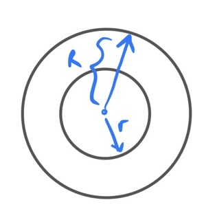
A family is (r,R,p,P) LSH if
\(Pr_{h \in H}[h(x) = h(y)] \geq p \ if\ d(x,y) \leq r\)
\(Pr_{h \in H}[h(x) = h(y)] \geq P \ if\ d(x,y) \geq R\)
If points are closer than the lower radius collision probability is higher and if the points are farther than the greater radius, collision probability is lower!
Jaccard similarity follows Gap LSH!
L2 Norm
\(d(x,y) = \sqrt{\sum_{i}(x_{i} - y_{i})^{2}}\)
u = random unit norm vector, w \(\in\) R parameter, b \(\sim\) Unif[0,w]
\(h(x) = \lfloor \frac{u.x + b}{w} \rfloor\)
If \(|x - y|_{2} < \frac{w}{2}\) , the probability that they will fall in separate partitions is low (x and y are close to each other)!
If \(|x - y|_{2} > 4w\) , the probability that they will fall in the same partition is low (x and y are far apart)!
Solving the near neighbour
(r,c) - near neighbour problem
-> Given query point q, return all points p such that \(d(p,q) < r\) and none such that \(d(p,q) > cr\)
-> Solving this gives a subroutine to solve the “nearest neighbour”, by building a data-structure for each r, in powers of \((1 + \epsilon)\)
How to actually use
We need to amplify the probability of collisions for close points since the graph of collision probability versus distance goes down smoothly for Jaccard distance.
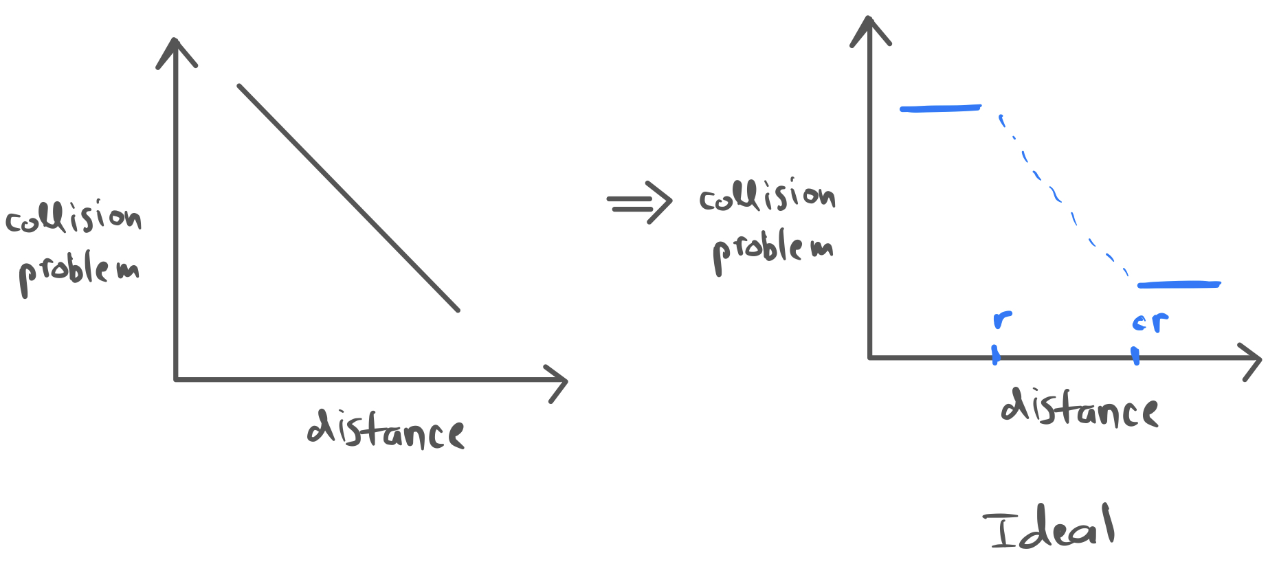
So, we want high value of collision probability if distance is less than \(r\) and low value if distance is greater than \(cr\) where \(c\) is some constant!
Band Construction
AND-ing of LSH
-> Define a composite function \(H(x) = (h_{1}(x),...,h_{k}(x))\)
-> \(Pr[H(x) = H(y)] = \Pi_{i}Pr[h_{i}(x) = h_{i}(y)] = Pr[h_{1}(x) = h_{1}(y)]^{k}\)
OR-ing
-> Create L independent hash-tables for \(H_{1},H_{2},...H_{L}\)
-> Given query q, search in \(\cup_{j} H_{j}(q)\)
Why is it better
Consider q,r with \(Pr[h(q) = h(y)] = 1 - d(q,y)\)
Probability of not finding y as one of the candidates in \(\cup_{j} H_{j}(q)\) is \(1 - (1 - (1-d)^{k})\)
Creating an LSH
-> If we have \((r,cr,p,q) LSH\)
-> For any y, wih \(|q - y| < r\)
Probability of y as candidate in \(\cup_{j}H_{j}(q) \geq 1 - (1-p^{k})^{L} \geq 1 - \frac{1}{e}\)
-> For any z, \(|q - z| > cr\)
Probability of z as candidate in any fixed \(H_{j}(q) \leq q_{k}\)
Expected number of such \(z \leq Lq^{k} \leq L = n^{\rho}\)
Space used = \(n^{1 + \rho}\)
Query time = \(n^{\rho}\)
We can show that for Hamming, angle etc, \(\rho \approx \frac{1}{c}\)
Therefore, we can get 2-approx near neighbours in \(O(\sqrt(n))\) query time
LSH : theory vs practice
In order to design LSH in practice, the theoretical parameter values are only a guidance, we need to search over the parameter space to find a good operating point!
Looking back
LSH is a tool for near neighbour problems
Trades off space with query time
Practical for medium to large datasets with fairly large number of dimensions, exceptions being sparse, very very high dimensional datasets
LSH (Locality Sensitive Hashing) Application
Finding Similar Items from a large Dataset with Precesion using LSH.
Intro
We want to search similar things from a large dataset. Brute Force approach takes O(N^2) time but LSH cuts this time to O(N)
Different Scenarios
While searching in the documents we can have two issues
1. We have a reasonable amount of Documents but every document have a large length.
2. We have a large number of documents with reasonable length.
Let's Explore the LSH usage in a large Documents Database
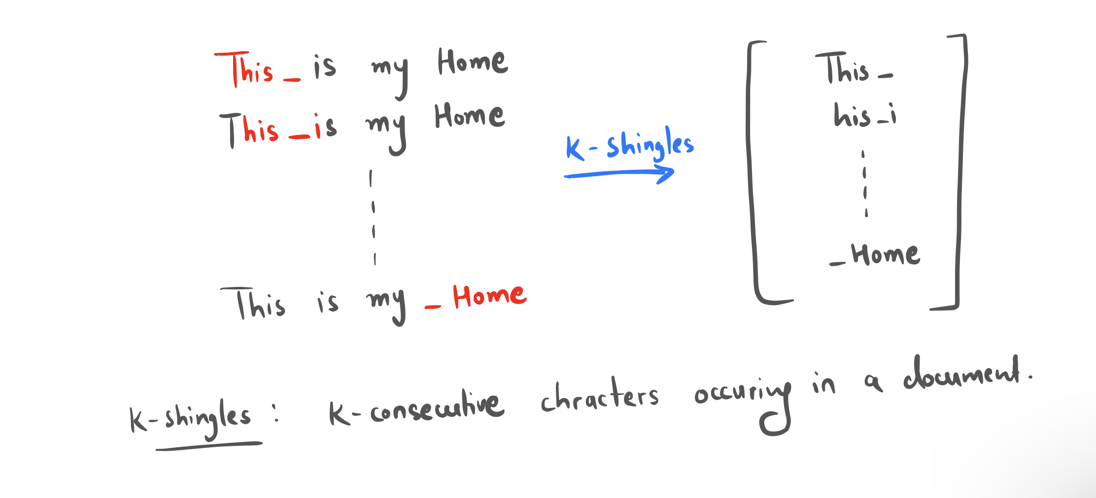
First we have to Vectorize the Document. To do that we build k-shingles. And then we make a big set of k-shingles and assign every shingle to an unique index
Now we have a large document of NXD dimensions with N documents and D columns having values 1/0 representing differnet shinngles. But we can't work with that dense matrix.
Before moving further, Let's see the Jacard Matrix
Now, we can take N documents of D dimensions and can find the Jaccard similarity above some threshold.
Now to overcome this issue of iterating through large N documents we use Min-Hashing.
For Example — Let suppose we have A = {1,0,0,1} and B = {0,0,0,1}. and let suppose these are shuffled already, the first index would be A[0]=1 and B[0]=0. A[0]!=B[0] which means the two are not similar and we return 0. Let's do the second shuffle. Shuffle gives A={0,0,1,1}, B={0,0,1,0}, so we get A[2]=B[2]!=0 which is a +1. Ultimately, if you shuffle enough times, you will find the similarity approaches the true value of 0.25. It is an approximation method that yields an expected similarity value. And more the data we have more the accuracy we'll generate.
Generating Unique Hashes
Take two random numbers a and b and pass through the forumula hash(x) = (a*x+b) mod D, where x is the index we are permuting. We generate new hashes by randomly choosing a, b.
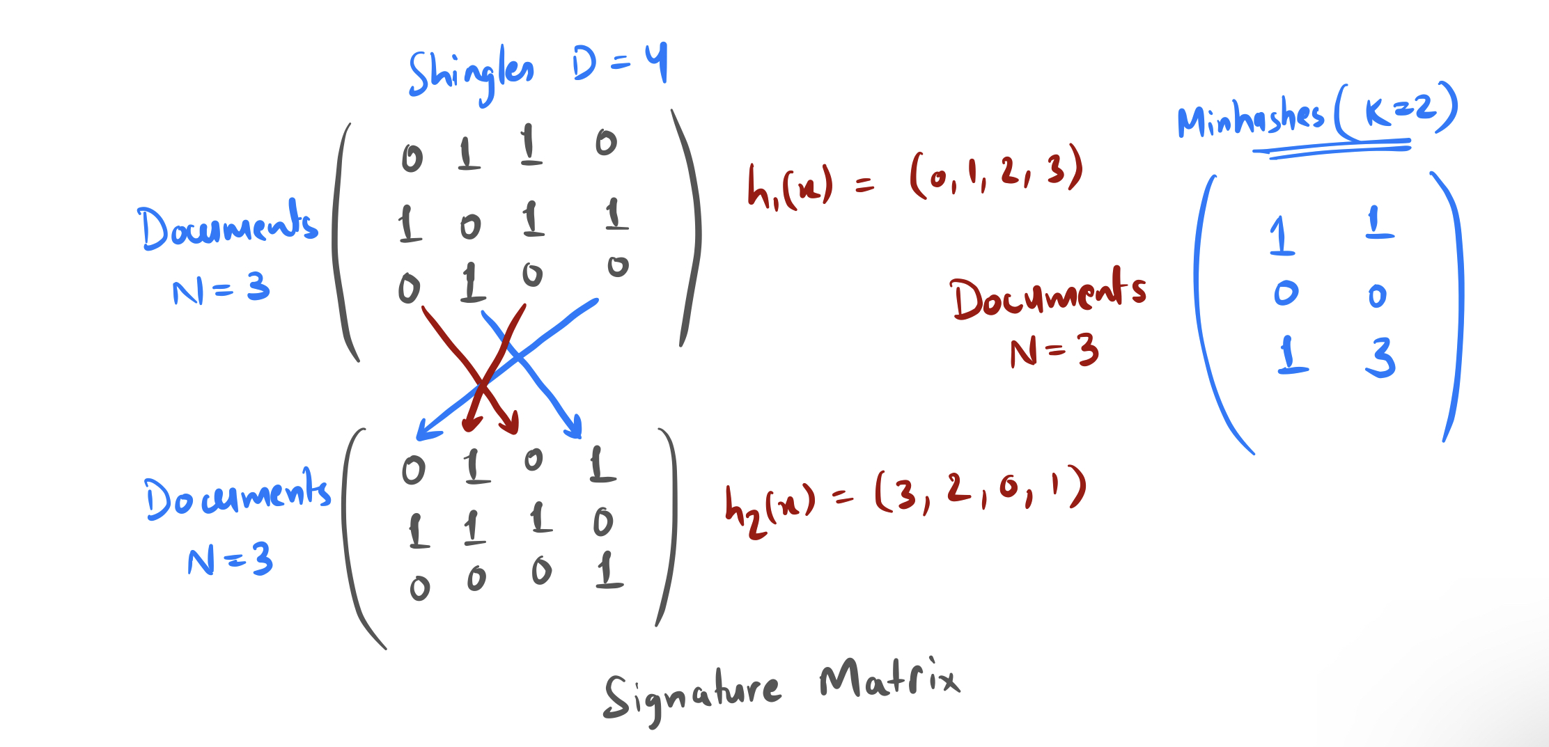
The Signature Matrix
Now we'll compute (N,K) Signature Matrix that has K number of random hash functions. Now we can compare N,K vectors as compared to the large N,D matrix. Signature matrix column represents one random hash functions. For every row in a column, the value is given by the index of the first nonzero element for that row (which is the MinHash).
Now, To write an efficient algorithm, we don’t actually need to permute all of the rows. It is now okay to just look at every element of the (N,D) dense matrix, and see if it has a 1, and if so if any permutations of the entry lead to a new MinHash.
Now instead of iterating on (N,D) we can iterate on (N,K) But it is still O(N^2)
Now to make it Precise we'll use LSH (Locality Sensitive Hashingh)
LSH: The band structure
Let's take an intuition that If we are able to map each row of the matrix to the buckets then the rows that are into the same bucket are somewhat similar or close. The “close” is precisely the desired similarity threshold we introduced earlier.
Now, coming to the defination of LSH, It is a family of functions which tune the functions such that points that are close to each other gets closer and points that are not close gets farthest apart with probability approaching to 1
Now we will take a band b. Earlier we were trying to match each row with other but now we give each row b possible chances. So we hash each row to b buckets and see who it matches with.
——> r below is the number of rows per band
Now, For better understanding, increasing b gives rows more chances to match, so it let’s in candidate pairs with lower similarity scores. Increasing r makes the match criteria stricter, restricting to higher similarity scores. r and b do opposite things or having a tradeoff between them (means one has opposite effect on the other one).
Now, we can precisely tune the parameters b and r such that we turn the likelihood of a candidate pair into a step function around our desired threshold
Note: Two rows are considered candidate pairs which means that they have the possibility to have a similarity score above the desired threshold, if the two rows have at least one band in which all the rows are identical.