.ipynb .pdf

repository open issue suggest edit

Binder Colab Live Code

Contents

Central Limit Theorem

---

Probability and Statistics - Recap

• Random experiments are experiments whose outcome cannot be predicted with certainty.

  • Tossing a coin

• Sample space is the set of all possible outcomes of a random experiment.

  • \(S = {H, T}\)

• An outcome is just an element of the sample space.

  • \(H\) is the outcome corresponding to getting a heads on a coin toss

• An event is a subset of the sample space.

  • \(A = {H}\) Event \(A\) occurs when you get a heads on a single coin toss

Random Variables

---

• Random variable is a function that maps the sample space to \(\mathbb{R}\) (real numbers).

  • \(x : S\) → \(\mathbb{R}\) (w is used to indicate an event)

\[\begin{split} x = \left\{ \begin{array}{lr} 1, & \text{if } w = \{H\}\\ 0, & \text{if } w = \{T\}\\ \end{array}\right\} \end{split}\]

• The cumulative distribution function (c.d.f) is a function \(F: \mathbb{R}\) → \([0,1]\) defined by \(F(x) = P(X <= x)\) where \(X\) is the random variable and \(x\) is an arbitary real number.

  • \(X\) ~ \(F\) indicates \(F\) is the distribution of r.v. \(X\)

  • \(P(a \lt X \le b) = P(X \le b) - P(X \le a) = F(b) - F(a)\)

  • \(P(X \lt a) = F(a^-)\)

Discrete and Continuous r.v.

• Discrete random variable - A random variable is said to be disrete if the set of all possible values of \(X\) is a sequence \(x_1, x_2 ... x_n\) (i.e. countable finite or infinite sequence)

• Continuous random variable - A random variable is said to be continuous if there exists a non-negative function such that the area under that curve for a particular region defines the probability of the random variable falling in that region.

	Discrete r.v.	Continuous r.v.
Function	Probability mass function	Probability density function
Range	\(p: \mathbb{R} \longrightarrow [0,1] \)	\( f: \mathbb{R} \longrightarrow [0,\infty) \)
p.m.f./ p.d.f.	\(p(x) = P(X = x)\)	\(P(X \in B) = \int_B f(x) dx\)
Summation/Integral	\(\sum_{i} p(x_i) = 1\)	\(\int_R f(x) dx = 1\)
Relation with c.d.f.	\(F(a) = \sum_{x_i <= a} p(x_i)\)	\(F(a) = \int_{-\infty}^{a} f(x) dx\)

Expectation

• Expectation is the average or mean value of a random variable.

	Discrete r.v.	Continuous r.v.
\(E[X]\)	\(\sum_{x} x.p(x)\)	\(\int_{R} x.f(x) dx\)

• Expectation of sum of random variables is equal to the sum of expectation of random variables, \(\textbf {irrespective of mutual independence}\), i.e.

\[ E[\sum_{i=1}^{n}X_i] = \sum_{i=1}^{n}E[X_i] \]

• \(E[c] = c\) where c is a constant

• \(E[cX] = cE[X]\) where c is a constant

Variance

• Variance of \(X\) is defined by \(Var(X) = E[(x-\mu)^2]\)

• Variance of sum of random variables is equal to the sum of expectation of random variables \(\textbf {only if all the random variables are mutually independent}\) i.e.

\[ Var(\sum_{i=1}^{n}X_i) = \sum_{i=1}^{n}Var(X_i) \]

• \(Var(c) = 0\)

• \(Var(X + c) = Var(X)\) where \(c\) is a constant

• \(Var(cX) = c^{2}Var(X)\) where \(c\) is a constant

Some common distributions

---

Consider \(X\) as the random variable.

Bernoulli

• In Bernoulli distribution, r.v. can take only two possible values 0 or 1 with \(X=1\) occuring with probability \(p\).

Distribution	Type	p.m.f	E[X]	Var(X)
Bernoulli	Discrete	\(p(x) = \left\{ \begin{array}{lr} 1-p, & \text{if x = 0}\\ p, & \text{if x = 1}\\ \end{array}\right\} \)	\(p\)	\(p(1-p)\)

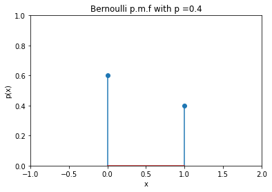
Fig. 4 Bernoulli distribution with \(p = 0.4\)

Binomial

• In n Binomial events, we can get the probability of getting \(r\) events \((r\le n)\) with favourable odds \(p\) and the rest with unfavourable odds \(q\) \((q = 1-p)\).

Distribution	Type	p.m.f	E[X]	Var(X)
Binomial	Discrete	\( p(r) = {n \choose r }p^{r}q^{n-r}\)	\(np\)	\(np(1-p)\)

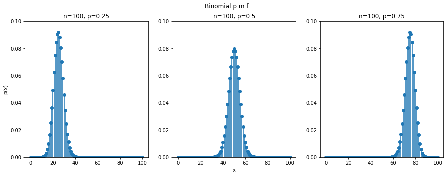
Fig. 5 Binomial distribution of 100 trials and \(p = 0.25\) (left), \(p = 0.5\) (middle), and \(p = 0.75\) (right)

Gaussian

• The normal/gaussian distribution can be expressed in terms of its expectation value and variance.

Distribution	Type	p.d.f	E[X]	Var(X)
Normal/Gaussian	Continuous	\( f(x) = \frac{1}{σ\sqrt{2Π}}\exp{(-\frac{1}{2}{(\frac{x-\mu}{σ})}^2)}\)	\(μ\)	\(σ\)

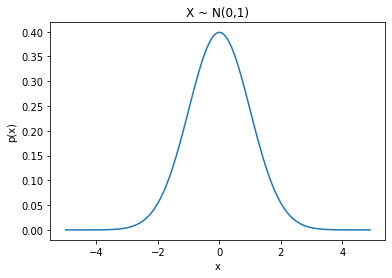
Fig. 6 Bell-shaped curve of the Gaussian distribution

Intuition for CLT

---

1. Probability distributions

Let’s say we want to explore the statistical properties of the heights of human adults. Let us divide the range of possible adult human heights, say from 4 feet to 7 feet, into bins of size 1 feet. We measure the height of a random person and put it in the corresponding bin; like a measurement of 5.6 feet goes into the bin [5 feet,6 feet). When we take multiple such measurements and stack them on top on each other in the respective bins, we get a histogram. This histogram tells us about the distribution of height among the people we measured. If we decrease our bin size and increase the number of measurements, we can make statements and estimates about the distribution more precisely.

However, it may happen one of the bin may remain empty as no measurment that we sampled fell in the range of that bin. However, that does not mean that no sample in the entire population will fall in that range. So, we use a curve to approximate the historgram and provide us with the same information. The advantage of a curve is that we can account for the empty bins and we do not need to take care of the bin size while sampling.

We don’t have enough money and time to sample the entire population. The curve approximated based on the mean and standard deviation of the data we collect is a good enough estimate for the entire population.

Takeaway

The probability distribution (as the name suggests) shows us how the probability of measurements is distributed.

We plot a histogram of the height data obtained from the Kaggle weight-height dataset and try to estimate a curve that fits the data.

import numpy as np
from scipy.stats import norm
import matplotlib.pyplot as plt
import pandas as pd

df = pd.read_csv("../assets/2022_01_10_central_limit_theorem_notebook/weight-height.csv")
arr = list(df['Height'])

# Fit a normal distribution to the data:
mu, std = norm.fit(arr)

# Plot the histogram.
plt.hist(arr, bins=25, density=True)

# Plot the PDF.
xmin, xmax = plt.xlim()
x = np.linspace(xmin, xmax, 100)
p = norm.pdf(x, mu, std)
plt.plot(x, p, 'k', linewidth=2)
title = '''Heights histogram
''' + "Fit results: mu = %.2f,  std = %.2f" % (mu, std)
plt.title(title)
plt.xlabel("Height x (inches)")
plt.ylabel("p(x)")
plt.show()

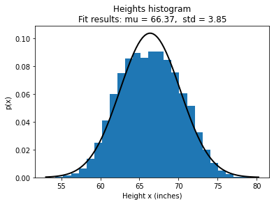
Fig. 7 Probability distribution of heights in the given dataset

2. Sampling a distribution

If we ask a computer to pick a measurment at random based on the probability described by the historgram/curve, it is likely to fall in the taller region of the histogram/curve. Every once in a while the computer will also pick some measurment from the shorter region of the histogram/curve.

Takeaway

Sampling a distribution (again as the name suggests) is getting samples from a distribution based on the probabilities described by the distribution.

Why do we have to sample from a distribution? We can use the computer to generate a lot of samples and we can plug them into various statistical tests and make inferences about the real-world data. Since we know the original distribution of the data we collect, we can compare our expectations of what will happen to what the reality is. So, sampling allows us to determine what statistical tests are capable of doing without doing much work in data collection.

3. Normal or Gaussian distribution

The normal or Gaussian distribution is a bell-shaped, symmetric curve. In the context of our adult human heights example, the x-axis represents the heights, and the y-axis represents the probability of observing someone of that height.

Properties

• The normal distributions are always centred at the average value.

• A tall, narrow curve means less range of the quantity on the x-axis

• The width of the curve is captured by the standard deviation \(\sigma\)

• Almost 68% of measurments fall within \(\pm 1 \sigma\)

• Almost 95% of the measurements fall within \(\pm 2 \sigma\)

• Almost 99.7% of the measurements fall within \(\pm 3 \sigma\)

• Given an average value and the standard deviation, we can draw a unique normal distribution.

• We observe this curve a lot in nature, such as for distributions of heights, weights, commute times, etc.

Central Limit Theorem

---

Even if you are not normal, the average is normal.

Let us take a uniform distribution in the range \(x \in [0, 1]\). The probability of picking any number in this range is uniform. We take 30 points at random from this range and call it sample 1. We calculate the mean of this sample and plot a histogram of the mean. We collect multiple such samples and plot their means on the histogram. When we take many such means, we see that the histogram represents the normal/Gaussian curve. Even when we have sampled the data from a uniform distribution, the means of the sampling distributions are normally distributed. Even when we begin with an exponential distribution, the means of the sampling distribution still end up being normally distributed.

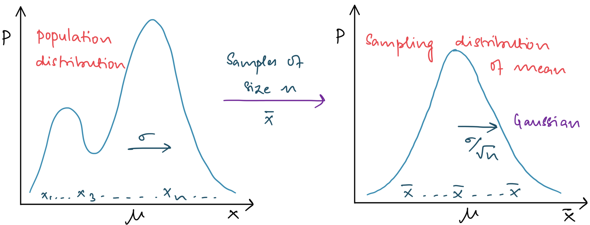
Fig. 8 Sampling distribution of the mean approaches the normal curve

Practical implications of the means being normally distributed

• In reality, we do not know what distribution our data belongs to. However, the CLT does not care about the original distribution of our data. So we do not have to worry about the distribution that the samples come from.

CLT is the basis for a lot of statistics. The normally distributed means are used to make confidence intervals and in various other statistical tests that help differentiate between two or more samples.

Caution

Few data scientists believe that the CLT is applicable only when we take a sample size \(\geq\) 30.

Formal Statement of CLT

---

Let \(X_1, X_2, ... . , X_n\) be \(n\) independent and identically distributed random variables with mean \(\mu\) and standard deviation as \(\sigma\). We introduce a new random variable \(S_n\) defined as:

\[S_n = \sum_i^n X_i\;\;,\;\; \overline{X}_n=\frac{S_n}{n}\]

Since they are independent and identically distributed random variables, the expectation and variance of \(S_n\) and \(\overline{X}_n\) is given as:

\[E(S_n)=n\mu \;\;\;\; , \;\;\;\; Var(S_n)=n\sigma^2\]

\[E(X_n)=\mu \;\;\;\; , \;\;\;\; Var(X_n)=\sigma^2/n\]

According to CLT:

\[\sqrt{n}(S_n-\mu) \xrightarrow{\text{distribution goes to}} N(0,\sigma^2)\]

As \(n\) increases, the distribution approaches standard normal distribution, \(N(0,1)\). By normalising \(S_n\), we get:

\[Z_n= \frac{S_n-n\mu}{\sqrt{n\sigma^2}}=\frac{S_n-n\mu}{\sigma\sqrt{n}} \xrightarrow[\text{converges to}]{\text{distribution}} N(0,1)\]

Or simply (for sufficiently large \(n\)):
\(S_n\approx N(n\mu,n\sigma^2)\)
\(X_n\approx N(\mu,\sigma^2/n)\)
\(Z_n\approx N(0,1)\)

Takeaway

As number of samples (\(n\)) increases, the distribution approaches Gaussian distribution.

Galton Board Experiment - An Application of CLT

---

The Galton board, invented by Francis Galton is a nice example to illustrate Central Limit Theorem (CLT). It demonstrates how a binomial distribution with a fairly large sample size can be approximated as a normal distribution.
Below is an image of a Galton Board (source):

Fig. 9 Galton Board Experiment [Source]

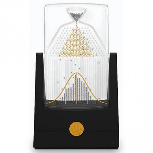
Consider \(n\) balls in the Galton Board. For each ball, it can go into \(k\) many bins. At each peg, it can either bounce to the left or right. On a biased board, let the probability of bouncing to the right be \(p\). Therefore, the probability of bouncing to the left is \(1-p\) (since the ball can not go straight down). Therefore, the probability of a ball to reach the \(k^{th}\) bin is given as:

\[ \binom nk \times p^k \times (1-p)^{(n-k)} \]

For a unbiased board, \(p=0.5\)

Accoding to CLT, the binomial distribution illustrated above can be approximated as a normal distribution, when the number of balls and pegs is very large; a condition satisfied by a Galton Board.

previous

Object Representations

next

Markov and Chebyshev Inequalities