Graph Laplacian and its Eigenvalues¶

Laplacian Matrix¶

Given a graph $ G = (V,E) $ where $ V = \{ v_1, v_2, ..., v_n \} $ is the set of nodes and $ E = \{ e_1, e_2, ..., e_n \} $ is the set of edges then Laplacian Matrix is defined as

\[ L = D - A \]

where $ A $ is an adjacency matrix

\[\begin{split} A_{i, j} = \begin{cases} 1, \text{if there is an edge between } v_i \text{ and } v_j\\ 0, \text{otherwise} \end{cases} \end{split}\]

and $ D $ is a diagonal matrix

\[\begin{split} D_{i, j} = \begin{cases} degree(v_i), \text{ if } i \text{ == } j\\ 0, \text{otherwise} \end{cases} \end{split}\]

$\rightarrow \text{If edges of graph are weighted then } degree(v_i) = \sum_j A_{ij}\\$

Consider the following example

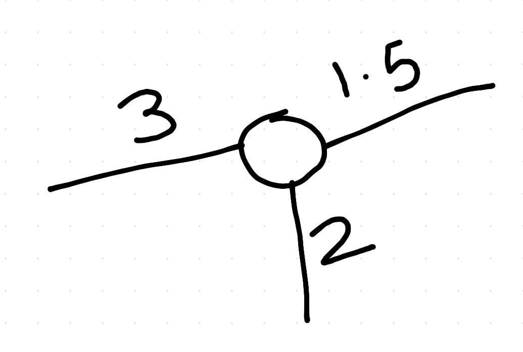
Fig. 26 Node with weighted edges¶

As we can see from the above figure, the edges of the node are weighted. So the degree of the node will be 3+2+1.5=6.5 rather than 3.

For irregular graphs we typically normalize $ L $ as

\[ L = D^{-1/2}LD^{-1/2} = I - D^{-1/2}AD^{-1/2} \]

where $ D^{-1/2} \equiv $ diagonal matrix with $ i^{th} $ entry $ = \frac{1}{\sqrt{d_i}} $

Diagonal entries, $ L_{ii} = d_i $
Offdiagonal entries, $$ L_{ij} = \begin{cases} 0, \text{ if there is no edge between } i \text{ and } j\\ -1, \text{otherwise} \end{cases} $$

$ \rightarrow $ Sum of each row of $ L $ is 0 as $ D_{ii} = \sum_{j=1}^{n}A_{ij} $ and $ L = D - A $

Eigenvector/Eigenvalues of Laplacian Matrix¶

$ \forall $ $ \lambda_i (\frac{1}{d} L) \in [0, 2] $

$ \lambda_i \in [0, 2d]$

$ \lambda_i (\frac{1}{d} L) \in [0, d] $

Normalized Laplacian = $ D^{-1/2}LD^{-1/2} $

For regular graphs (d)

\[\begin{split} D^{-1/2} = \begin{bmatrix} \frac{1}{\sqrt{d}} & & \\ & \ddots & \\ & & \frac{1}{\sqrt{d}} \end{bmatrix} = \frac{1}{\sqrt{d}} I \end{split}\]

Normalized Laplacian = $ (\frac{1}{\sqrt{d}} I) L (\frac{1}{\sqrt{d}} I) = \frac{1}{d}L $

$ \lambda_1(L) = 0 \\ $ $ \lambda_k(L) = 0 $ iff k disconnected components are present in graph

For example, consider the following graph

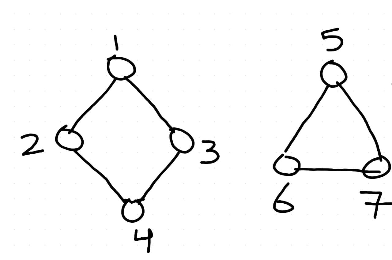
Fig. 27 A disconnected graph¶

\[\begin{split} A = \begin{bmatrix} 0 \hspace{2mm} 1 \hspace{2mm} 1 \hspace{2mm} 0 \hspace{2mm} 0 \hspace{2mm} 0 \hspace{2mm} 0 \hspace{2mm} \\ 1 \hspace{2mm} 0 \hspace{2mm} 0 \hspace{2mm} 1 \hspace{2mm} 0 \hspace{2mm} 0 \hspace{2mm} 0 \hspace{2mm} \\ 1 \hspace{2mm} 0 \hspace{2mm} 0 \hspace{2mm} 1 \hspace{2mm} 0 \hspace{2mm} 0 \hspace{2mm} 0 \hspace{2mm} \\ 0 \hspace{2mm} 1 \hspace{2mm} 1 \hspace{2mm} 0 \hspace{2mm} 0 \hspace{2mm} 0 \hspace{2mm} 0 \hspace{2mm} \\ 0 \hspace{2mm} 0 \hspace{2mm} 0 \hspace{2mm} 0 \hspace{2mm} 0 \hspace{2mm} 1 \hspace{2mm} 1 \hspace{2mm} \\ 0 \hspace{2mm} 0 \hspace{2mm} 0 \hspace{2mm} 0 \hspace{2mm} 1 \hspace{2mm} 0 \hspace{2mm} 1 \hspace{2mm} \\ 0 \hspace{2mm} 0 \hspace{2mm} 0 \hspace{2mm} 0 \hspace{2mm} 1 \hspace{2mm} 1 \hspace{2mm} 0 \hspace{2mm} \\ \end{bmatrix}\end{split}\]

$\hspace{7mm} \lambda_1(L) = 0 $ using all ones eigen vector $ \\ \hspace{7mm} \lambda_2(L) = 0 \\ $

\[\begin{split} \hspace{7mm} v_1 = \begin{bmatrix} 1 \\ 1 \\ 1 \\ 1 \\ 0 \\ 0 \\ 0 \end{bmatrix} \Rightarrow L.v_1 = \begin{bmatrix} 0 \\ 0 \\ 0 \\ 0 \\ 0 \\ 0 \\ 0 \end{bmatrix}\end{split}\]

\[\begin{split} \hspace{7mm} v_2 = \begin{bmatrix} 0 \\ 0 \\ 0 \\ 0 \\ 1 \\ 1 \\ 1 \end{bmatrix} \Rightarrow L.v_2 = \begin{bmatrix} 0 \\ 0 \\ 0 \\ 0 \\ 0 \\ 0 \\ 0 \end{bmatrix}\end{split}\]

$ \rightarrow v_1 $ and $ v_2 $ are orthogonal to each other.

$ \rightarrow $ Looking at the values of $ v_2(L), ...., v_k(L) $ tells us what the components are.

What if the graph is disconnected?¶

$ \hspace{7mm} \lambda_2(L) $ will still give a “measure of how much, $ G $ resembles a 2 disconnected components, i.e., sparsest cut”.

CS328-2022 Notes

Graph Laplacian and its Eigenvalues

Contents

Graph Laplacian and its Eigenvalues¶

Laplacian Matrix¶

Eigenvector/Eigenvalues of Laplacian Matrix¶

What if the graph is disconnected?¶